Monitoring Linux servers with Prometheus, Node Exporter and Grafana Time Series

I am writing this article to supplement one of my recent YouTube videos. In there, I provided a step-by-step tutorial to create a Grafana dashboard to monitor Linux servers. The data is collected by Node Exporter and stored in the Prometheus database.
Both, the video and this article, are complementing each other since some of the materials are better in a motion picture format and some shine brighter in the written word.
To get a better understanding of the topic, I recommend watching the video first and then getting back to this article. But the decision of what should go first is surely up to you.
Data flow
My dashboard visualizes server diagnostic data that is stored in the Prometheus database where it gets collected from the Node Exporters. Every node exporter works with one Linux server instance.
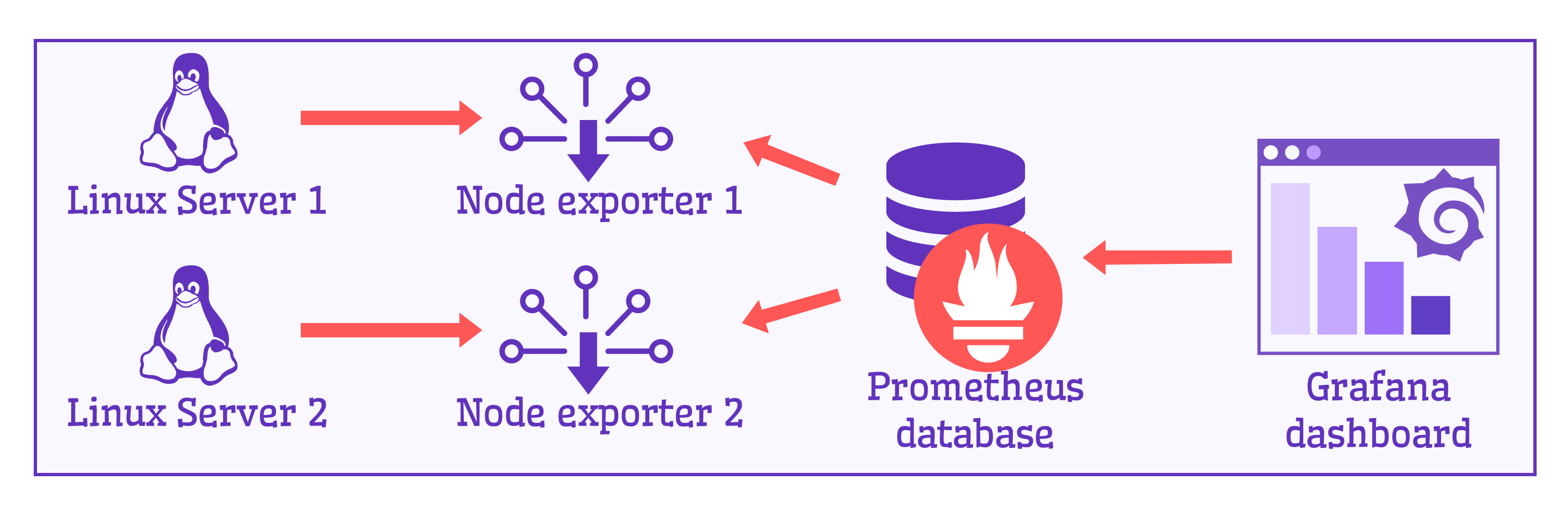
For more information on how such a system can be set up, please, refer to the Prometheus documentation for Node Exporter.
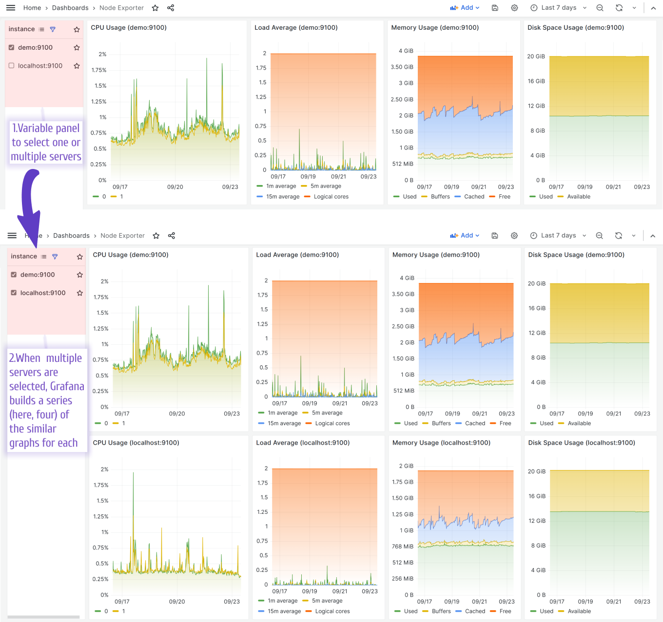
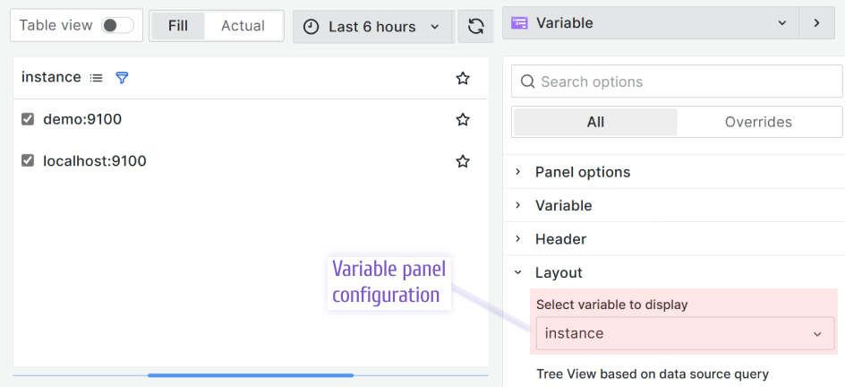
Variable panel
I started my dashboard by configuring a filtering functionality. To be more user-friendly, I wanted to position my filter on the same horizontal level as my Time Series.
There is only one Grafana plugin as of this moment that allows achieving such a requirement. It is the Business Variable panel.
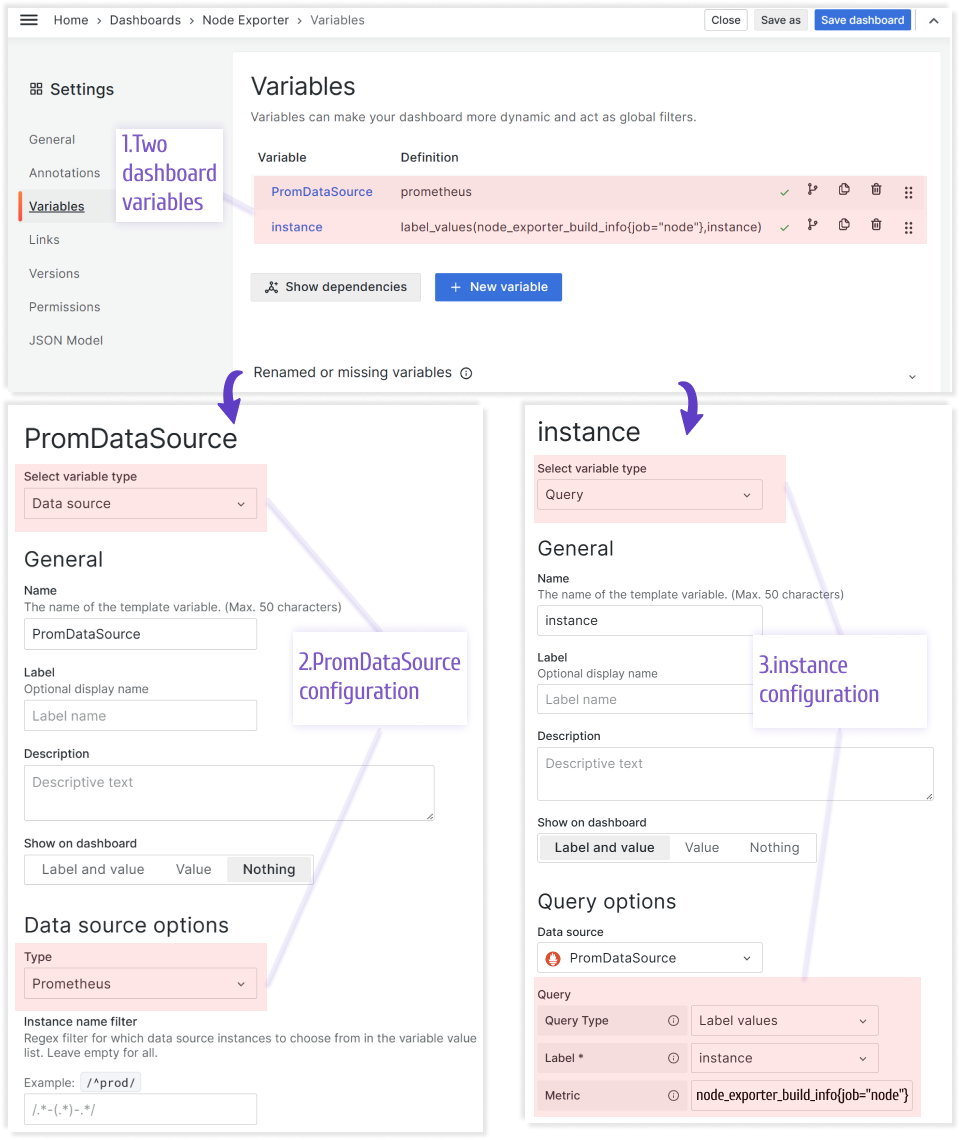
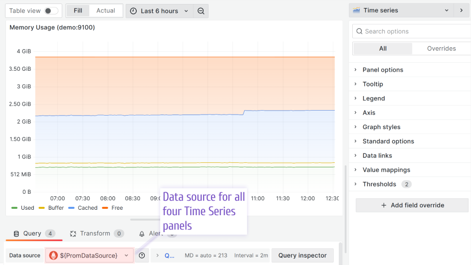
Data Source
All panels have the same data source to read data from. The data source is configured as a dashboard variable.
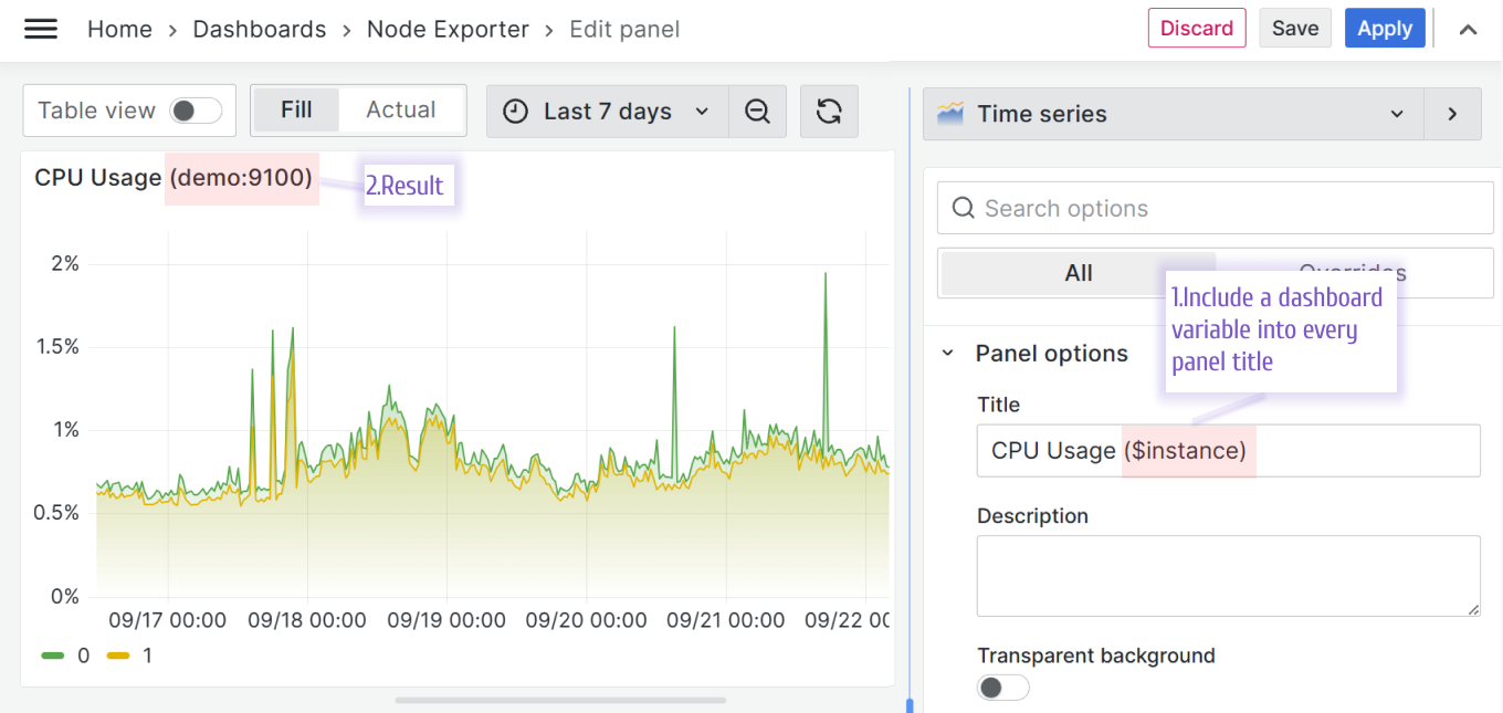
Dynamic Title
I made the Time Series panels' titles dynamic by including the dashboard variable {instance} in the value. That makes every title change according to the selected server on the variable panel.
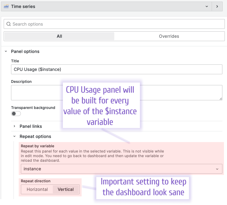
Repeat Options
The dashboard variable {$instance} that I created to have the filtering functionality represents an array of values. Each value is a server name.
According to my design, one server per chart should be displayed. What this means is when a user selects two servers in the variable panel, the same two charts should be created, one per server.
To archive that, in the Time Series edit mode, in the panel options category, you can specify which variable to use for the Repeat feature.
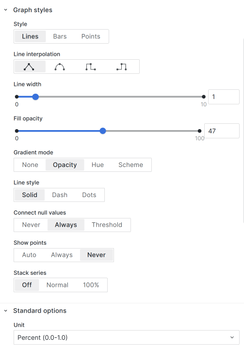
Visualization Options
By visualization option I mean the settings that a user configures on the right-hand side of any Grafana panel. The configuration in my case is almost identical for all four panels.
I already mentioned everything I changed in the Panel options category, namely, dynamic title and Repeat options. For the rest, I touched upon Graph styles and Standard option categories to set the fill opacity, gradient mode, and units.
Prometheus Queries
This dashboard consists of four time series for each selected server.
- CPU Usage
- Load Average
- Memory Usage
- Disk Space
CPU Usage
This panel contains one query to calculate the usage per CPU.
(
  (1 - rate(node_cpu_seconds_total{job="node", mode="idle", instance="$instance"}[$__interval]))
/ ignoring(cpu) group_left
  count without (cpu)( node_cpu_seconds_total{job="node", mode="idle", instance="$instance"})
)
Load Average
Query to compute the total number of active CPUs on the server.
count(node_cpu_seconds_total{job="node", instance="$instance", mode="idle"})
Query to compute the average 1-minute load.
node_load1{job="node", instance="$instance"}
Query to compute the average 5-minute load.
node_load5{job="node", instance="$instance"}
Query to compute the average 15-minute load.
node_load15{job="node", instance="$instance"}
Memory Usage
Query to retrieve used memory
(
  node_memory_MemTotal_bytes{job="node", instance="$instance"}
-
  node_memory_MemFree_bytes{job="node", instance="$instance"}
-
  node_memory_Buffers_bytes{job="node", instance="$instance"}
-
  node_memory_Cached_bytes{job="node", instance="$instance"}
)
Query to retrieve buffer memory
node_memory_Buffers_bytes{job="node", instance="$instance"}
Query to retrieve cached memory
node_memory_Cached_bytes{job="node", instance="$instance"}
Query to retrieve free memory
node_memory_MemFree_bytes{job="node", instance="$instance"}
Disk Space
Query to retrieve used memory
sum(
  max by (device) (
    node_filesystem_size_bytes{job="node", instance="$instance", fstype!=""}
  -
    node_filesystem_avail_bytes{job="node", instance="$instance", fstype!=""}
  )
)
Query to retrieve available memory
sum(
  max by (device) (
    node_filesystem_avail_bytes{job="node", instance="$instance", fstype!=""}
  )
)
Let’s Stay Connected!
Join the Conversation: Stay updated and share your thoughts! Subscribe to our YouTube Channel and leave your comments—we can’t wait to hear what you think.
Your input helps us improve, so don’t hesitate to get in touch!